The Basics of Spatial Filters

A digital image consists of rows and columns of pixels. Each pixel has a discrete intensity value. For example, an 8-bit image has the intensity of each pixel defined by an 8-bit integer (values 0 to 255), with 0 being black and 255 being white and all the values are some level of grey between black and white. The spacial domain of a digital image is simply defined as the x-y plane of pixels that make up that image. Spacial Filters operate within this domain and can be expressed as follows:

g(x,y) = T[f(x,y)]

where g(x,y) is the filtered image, f(x,y) is the original image, and T is the transformation that operates on the neighborhood of the point (x,y).

The neighborhood of a point (x,y) contains useful local information for filtering an image. A convolution kernel is a 2D operator with a size that defines this neighborhood. For example, a 3x3 kernel  defines the neighboring pixels as the immediate N, NE, E, SE, S, SW, W, and NW pixels around and including the pixel (x,y) being operated on (Figure 1). Other kernel sizes are 5x5, 7x7 and so on. The size of a kernel can be as large as is needed but should be kept to a size that contains the useful information to be extracted.

Figure 1: 3x3 neighborhood of point (x,y) in an image

A convolution kernel recalculates the value of a pixel (x,y) by using the value of the pixel (x,y) and weighing it against the neighboring pixel values by use of coefficients. For example, the coefficients a, b, c, d, e, f, g, h, and x below define the coefficients of a 3x3 kernel:

A	B	C
D	X	E
F	G	H

3x3 Convolution Kernel

The following convolution kernel applied to an image is then just the original image, as the coefficient for each surrounding neighbor of the pixel (x,y) is 0 and the pixel (x,y) in the center has the identity of 1, or the original pixel value.

0	0	0
0	1	0
0	0	0

Identity 3x3 Kernel

Modifying the coefficients of the kernel will make use of neighboring pixel information to lesser or greater extents, produce geometric information, and compute changes in intensity (derivatives or gradients). Look for example at the following simple Prewitt Filters below. The first one modifies the original image by making use of the pixels to the NorthEast and SouthWest of each (x,y) pixel in the image, and also does not include the pixel (x,y) in the modified image. The result is essentially highlighting the gradient in the SW direction of the image. The line in the lower right circle that runs from the NorthEast  to the SouthWest has mostly disappeared as it each of the pixels along this line or feature has no gradient along this direction of the filter. The second Prewitt filter makes use of information only from the pixel to the immediate right and left of every pixel in the image, and the coefficient of -1 on the left and coefficient of 1 on the right is a gradient that highlights changes in intensity along the horizontal axis. The result is that horizontal lines in the original image disappear. In this way, a convolution kernel can produce geometrical information as well as gradient information in an image.

Figure 2: Left - original image. Center - Prewitt 3x3 SW Filter. Right - Prewitt 3x3 East Filter.

 

0	-1	-1
1	0	-1
1	1	0

3x3 Prewitt Filter for SW Gradient

0	0	0
-1	0	1
0	0	0

3x3 Prewitt Filter for E Gradient

Figure 3: Left - original image. Right - Prewitt Filter Showing Gradients

If the original pixel information were included in the convolution kernel (i.e. a non-zero value in the center of the kernel), a gradient filter would have the effect of sharpening edges in an image. The following shows the sharpening effect and the convolution kernel of the spatial filter that was applied:

Figure 4: Left - Original Image. Right - 5x5 convolution kernel applied for sharpening

 

-1	-1	-1	-1	-1
-1	-1	-1	-1	-1
-1	-1	30	-1	-1
-1	-1	-1	-1	-1
-1	-1	-1	-1	-1

5x5 Kernel used for Sharpening

A spacial filter is then a 2D Kernel applied to every point (x,y) in an image. Spacial filters have the effect of sharpening or smoothing (blurring) sharp edges in an image. This is typically denoted as highpass and lowpass filtering. Some common highpass and lowpass special filters are as follows:

Type		Filters
Highpass	Gradient, Laplacian, Prewitt, Sobel, Roberts
Lowpass	Gaussian, Median, Lowpass

The Gaussian Filter is particularly useful for reducing the effect of random noise in images, usually caused by electronic noise in the imaging sensor. The Gaussian curve has many special mathematical properties that makes it useful in statistics, Fourier analysis, and in this case, image processing. Symmetrical at its center, the Gaussian curve quickly falls off and can be represented discretely as a convolution kernel in which the coefficients of the surrounding pixels are all taken into account as a Gaussian distribution. The effect of the Gaussian filter then is essentially local averaging.

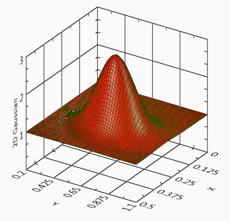Figure 5: 2D Gaussian Curve Shape

5x5 Gaussian Kernel

Electronic noise in an image often appears as a small uneven distribution of pixel intensity in an image where an even intensity would be expected. For example, the following shows an image on the left with random noise and a rather uneven intensity. The processed image on the right had a 3x3 Gaussian Filter applied to it.

Figure 6: Left - Original Image with Noise. Right - Processed Image using a 3x3 Gaussian Filter.

 As can be seen, the Gaussian filter does an excellent job reducing random noise in an image! A frequent problem that exists with the Gaussian distribution as a local averaging filter, however, is that it tends to blur useful edge information. One way to reduce this effect is to use a Median Filter instead. The Median Filter has a specified kernel size that replaces the pixel x,y being processed with the median of the neighboring pixels. The median filter, in effect, reduces image noise while still preserving edge information.